Cell & Cell Reference and cell Referencing (Addressing)

Cell

1.      A cell is the intersection between a row and a column on a spreadsheet that starts with cell A1. In the following example, a highlighted cell is shown in a Microsoft Excel spreadsheet. D8 (column D, row 8) is the highlighted cell. Any modifications made while this cell is highlighted will be limited to this item in the spreadsheet.

Here, D8 is the active cell. In the formula bar, you can see that the cell content is =SUM (D2:D5). This formula evaluates to the result of $162.00 by calculating the sum of the values stored in cells D2 through D5.

Each cell in a spreadsheet can contain any value that can be called using a relative cell reference or called upon using a formula.

Cell References

Relative Reference | Absolute Reference | Mixed Reference

Cell references in Excel are very important. Understand the difference between relative, absolute and mixed reference, and you are on your way to success.

Relative Reference

By default, Excel uses relative references. See the formula in cell D2 below. Cell D2 references (points to) cell B2 and cell C2. Both references are relative.

Cell D3 references cell B3 and cell C3. Cell D4 references cell B4 and cell C4. Cell D5 references cell B5 and cell C5. In other words: each cell references its two neighbors on the left.

Absolute Reference

See the formula in cell E3 below.

1. To create an absolute reference to cell H3, place a $ symbol in front of the column letter and row number ($H$3) in the formula of cell E3.

The reference to cell H3 is fixed (when we drag the formula down and across). As a result, the correct lengths and widths in inches are calculated.

Mixed Reference

Sometimes we need a combination of relative and absolute reference (mixed reference).

1. See the formula in cell F2 below.

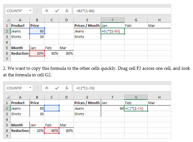
Do you see what happens? The reference to the price should be a fixed reference to column B. Solution: place a $ symbol in front of the column letter ($B2) in the formula of cell F2. In a similar way, when we drag cell F2 down, the reference to the reduction should be a fixed reference to row 6. Solution: place a $ symbol in front of the row number (B$6) in the formula of cell F2.

Result:

Note: we don't place a $ symbol in front of the row number of $B2 (this way we allow the reference to change from $B2 (Jeans) to $B3 (Shirts) when we drag the formula down). In a similar way, we don't place a $ symbol in front of the column letter of B$6 (this way we allow the reference to change from B$6 (Jan) to C$6 (Feb) and D$6 (Mar) when we drag the formula across).

3. Now we can quickly drag this formula to the other cells.

The references to column B and row 6 are fixed.